movAv.m
(see also movAv2 - an updated version allowing weighting)
Description
Matlab includes functions called movavg and tsmovavg ("time-series moving average") in the Financial Toolbox, movAv is designed to replicate the basic functionality of these. The code here provides a nice example of managing indexes inside loops, which can be confusing to begin with. I've deliberately kept the code short and simple to keep this process clear.
movAv performs a simple moving average that can be used to recover noisy data in some situations. It works by taking an the mean of the input (y) over a sliding time window, the size of which is specified by n. The larger n is, the greater the amount of smoothing; the effect of n is relative to the length of the input vector y, and effectively (well, sort of) creates a lowpass frequency filter - see the examples and considerations section.

Because the amount of smoothing provided by each value of n is relative to the length of the input vector, it's always worth testing different values to see what's appropriate. Remember also that n points are lost on each average; if n is 100, the first 99 points of the input vector don't contain enough data for a 100pt average. This can be avoided somewhat by stacking averages, for example, the code and graph below compare a number of different length window averages. Notice how smooth 10+10pt is compared to a single 20pt average. In both cases 20 points of data are lost in total.
% Create xaxis
x=1:0.01:5;
% Generate noise
noiseReps = 4;
noise = repmat(randn(1,ceil(numel(x)/noiseReps)),noiseReps,1);
noise = reshape(noise, 1, length(noise)*noiseReps);
% Generate ydata + noise
y=exp(x)+10*noise(1:length(x));
% Perfrom averages:
y2 = movAv(y, 10); % 10 pt
y3 = movAv(y2, 10); % 10+10 pt
y4 = movAv(y, 20); % 20 pt
y5 = movAv(y, 40); % 40 pt
y6 = movAv(y, 100); % 100 pt
% Plot
figure
plot(x,[y', y2', y3', y4', y5', y6'])
legend('Raw data', '10pt moving average', '10+10pt', '20pt', '40pt', '100pt')
xlabel('x');
ylabel('y');
title('Comparison of moving averages')

function output = movAv(y,n)
The first line defines the function's name, inputs and outputs. The input x should be a vector of data to perform the average on, n should be the number of points to perform the average over output will contain the averaged data returned by the function.
% Preallocate output
output=NaN(1,numel(y));
% Find mid point of n
midPoint = round(n/2);
The main work of the function is done in the for loop, but before starting two things are prepared. Firstly the output is pre-allocated as NaNs, this served two purposes. Firstly preallocation is generally good practice as it reduces the memory juggling Matlab has to do, secondly, it makes it very easy to place the averaged data into an output the same size as the input vector. This means the same xaxis can be used later for both, which is convenient for plotting, alternatively the NaNs can be removed later in one line of code (output = output(~isnan(output));
The variable midPoint will be used to align the data in the output vector. If n=10, 10 points will be lost because, for the first 9 points of the input vector, there isn't enough data to take a 10 point average. As the output will be shorter than the input, it needs to be aligned properly. midPoint will be used so an equal amount of data is lost at the start and end, and the input is kept aligned with the output by the NaN buffers created when preallocating output.
for a = 1:length(y)-n
% Find index range to take average over (a:b)
b=a+n;
% Calculate mean
output(a+midPoint) = mean(y(a:b));
end
In the for loop itself, a mean is taken over each consecutive segment of the input. The loop will run for a, which is defined as 1 up to the length of the input (y), minus the data that will be lost (n). If the input is 100 points long and n is 10, the loop will run from (a=) 1 to 90.
This means a provides the first index of the segment to be averaged. The second index (b) is simply a+n-1. So on the first iteration, a=1, n=10, so b = 11-1 = 10. The first average is taken over y(a:b), or x(1:10). The average of this segment, which is a single value, is stored in output at index a+midPoint, or 1+5=6.
On the second iteration, a=2. b= 2+10-1 = 11, so the mean is taken over x(2:11) and stored in output(7). On the last iteration of the loop for an input of length 100, a=91, b = 90+10-1 = 100 so the mean is taken over x(91:100) and stored in output(95). This leaves output with a total of n (10) NaN values at index (1:5) and (96:100).
Examples and considerations
Moving averages are useful in some situations, but they're not always the best choice. Here are two examples where they're not necessarily optimal.
Microphone calibration
This set of data represents the levels of each frequency produced by a speaker and recorded by a microphone with a known linear response. The output of the speaker varies with frequency, but we can correct for this variation with the calibration data - the output can be adjusted in level to account for the fluctuations in the calibration.

Notice that the raw data is noisy - this means that a small change in frequency appears to require a large, erratic, change in level to account for. Is this realistic? Or is this a product of the recording environment? It's reasonable in this case to apply a moving average that smooths out the level/frequency curve to provide a calibration curve that is slightly less erratic. But why isn't this optimal in this example?
More data would be better - multiple calibrations runs averaged together would destroy the noise in the system (as long as it's random) and provide a curve with less subtle detail lost. The moving average can only approximate this, and may remove some higher frequency dips and peaks from the curve that truly do exist.
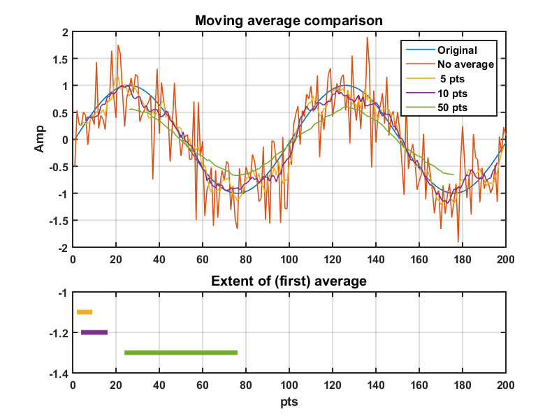
Sine waves
Using a moving average on sine waves highlights two points:
- The general issue of choosing a reasonable number of points to perform the average over.
- It's simple, but there are more effective methods of signal analysis than averaging oscillating signals in the time domain.
An alternative approach would be to construct a lowpass filter than can be applied to the signal in the frequency domain. I'm not going to go into detail as it goes beyond the scope of this article, but as the noise is considerably higher frequency than the waves fundamental frequency, it would be fairly easy in this case to construct a lowpass filter than will remove the high frequency noise.
No comments:
Post a Comment