Introduction to psychometric curves and fitting a simple psychometric function

Code
GitHub: Matlab code and Python package

Introduction
An important aim of psychophysics is to quantify the relationship between stimulus parameters and an observer's subjective appreciation of what's going on. Signal detection theory approaches this problem by attributing perceptual sensitivity to thresholds that act at multiple levels in a system. In this context, a threshold could, for example, be how loud a sound needs to be to determine its location to a certain degree of accuracy, or how long a light needs to be on to determine its direction of movement. Above threshold, and the task is possible to a certain degree of accuracy. Below threshold and it's not possible to discriminate as accurately.

Experimentally, thresholds are often measured in two-alternative forced choice (2AFC) tasks or in go-no go paradigms (GNG). In 2AFC tasks a subject is asked to indicate one of two choices in response to a stimulus. For example, indicate white if a colour appears white, or black if it appears black in response to a shade of grey. Alternatively, GNG tasks require a subject to not respond ("no go") until a stimuli meets a certain criteria, then respond ("go").

In both of these types of task, a subjects performance can be measured as a function of the stimulus parameters - either as % correct, or similar, in 2AFC or d' in GNG, where d' is a function of hits, misses, and false alarms. Regardless of the exact metric used, the subjects performance can be described by two main parameters; bias (the "point of subject equality", PSE) and discrimination sensitivity (as in ability to discriminate between two conditions, such as white and black).

For example, imagine a subject performing a 2AFC task where they're presented with a shade of grey and they have to press one button to categorise the colour as white, or another button to categorise the colour as black. Intuitively, they're more likely to classify a grey stimulus as black the closer it is to black, and less likely the colour it is to white. So plotting their responses as a proportion of black responses (y) against the stimuli presented (x). We could use this sort of task to see how other factors, like the colour of a background, could affect perception of the shade of grey.

Fitting a psychometric curve
Psychometric curves are models fit to the experimental data that describe the subjects behaviour and give quantitative estimates of their discrimination sensitivity and bias. This function, FitPsycheCurveLogit, is designed to fit a basic psychometric curve using a general linear model with a logit link function. The fitted curve will allow us to calculate the bias and discrimination sensitivity of the subject under various conditions.

FitPsycheCurveLogit takes up to 4 inputs; the x axis (xAxis), the subjects response (yData), the n value for each point (weights), and targets. weights should be the same length as yData and xAxis.
The function returns the coefficients of the fitted psychometric curve (coeffs), the stats for this fit (stats) the curve itself generated on a higher resolution x axis (curve, where curve(:,1) = the higher res x axis and curve(:,2) = the curve itself). Additionally, the optional input targets can contain performance thresholds (y data points) at which to evaluate the curve and return the corresponding x values (in the output thresholds). This is useful for calculating the bias and discrimination sensitivity from the fitted model. targets should be specified in the range 0 to 1.

For weighted fits it's important to understand how glmfit expects weights to be specified. yData should be the number of successes and weights to be the total number (n) of trials. This is essential to bear in mind when trying to do a weighted fit to data where you have, say % correct values, each with different n. In this case yData should be the number of correct trails, not the actual % correct value, ie. (%Correct/100) * n. This doesn't matter so much for unweighted fits where weights can be specified as all 1s; in this case, each point is given equal weight and yData can be specified as  (%Correct/100) * 1, or simply %Correct/100. Or, alternatively, if all the weights are specified as 100, yData could be (%Correct/100) * 100, or simply %Correct.

Let's generate some more data, fit some curves, and calculate the bias and threshold under different conditions. Imagine we have the following conditions in which we want to test the subjects ability to discriminate between the colours white and black:

• Neural background - the "default" condition with no distractions.
• Dark background - the target stimulus is presented with a dark background that contrasts with white stimuli, perhaps making them look whiter. This increases the subjects likelihood of categorising a stimulus as white, and creating a bias (at least it does in our made up data anyway!).
• Obscured target - the stimulus is obscured in some way, making the task harder and increasing the subjects threshold (decreasing discrimination sensitivity); meaning a greater difference in shade would be required to make the white/black categorisation as accurately as in the default condition. 

% Make up some data

x=1:10

yNeutralBg = [5, 5, 10, 20, 40, 60, 80, 90, 95, 95]/100

yDarkBg = [0, 0, 2.5, 5, 10, 20, 40, 60, 80, 90]/100

yObscured = [25, 25, 30, 35, 45, 55, 65, 70, 75, 75]/100

% Plot the made up data

figure, scatter(x,yNeutralBg)

hold on

scatter(x,yDarkBg)

scatter(x,yObscured)

ylabel('Proportion "black" responses')

xlabel('Greyscale, 1=white, 10=black')

% Fit psychometirc functions

targets = [0.25, 0.5, 0.75] % 25%, 50% and 75% performance

weights = ones(1,length(x)) % No weighting

% Fit for neutral background

[coeffsNeutralBg, ~, curveNeutralBg, thresholdNeutralBg] = ...

    FitPsycheCurveLogit(x, yNeutralBg, weights, targets);

% Fit for dark background

[coeffsyDarkBg, ~, curveDarkBg, thresholdDarkBg] = ...

    FitPsycheCurveLogit(x, yDarkBg, weights, targets);

% Fit for obscured target

[coeffsObscured, ~, curveObscured, thresholdObscured] = ...

    FitPsycheCurveLogit(x, yObscured, weights, targets);

% Plot psychometic curves

plot(curveNeutralBg(:,1), curveNeutralBg(:,2), 'LineStyle', '--')

plot(curveDarkBg(:,1), curveDarkBg(:,2), 'LineStyle', '--')

plot(curveObscured(:,1), curveObscured(:,2), 'LineStyle', '--')

legend('Neutral background', 'Dark background', 'Obscured target', ...

'Neutral background fit', 'Dark background fit', 'Obscured target fit');

Note that in this code the fit is unweighted and FitPsycheCurveLogit is passed proportional yData with a range 0 to 1, so weights is specified as all ones. If yData was left as % (by not dividing by 100 when creating the data), weights should be specified as all 100s.

Immediately it becomes obvious that the subject's response differs depending on the experimental conditions. It's also obvious one of the fits does not seem to fit its data quite as well as the other two (the data points from the obscured target condition appear to deviate for its fit more).

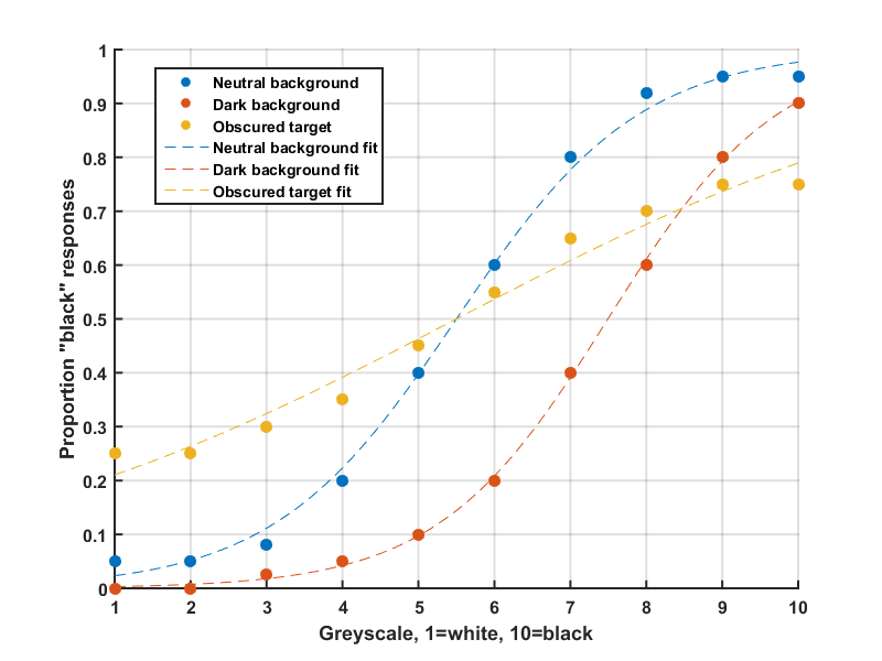
Qualitatively, we can see that the dark background has shifted the psychometric curve to the right - showing a bias to respond "white". The curves for the two non-obscured conditions also have steeper slopes than the obscured condition, indicating better discriminations sensitivities in these conditions compared to the obscured condition. In other words, a lesser change in colour is required in unobscured conditions for the same level of discrimination to occur compared to the harder obscured condition.

Let's quantify the differences in sensitivity and bias. Unfortunately, the logit fit does not immediately return coefficients that correspond to these values, but they're fairly trivial to calculate from the values returned by FitPsycheCurveLogit. In the above code, the fit is run with targets=[0.25, 0.5, 0.75]. The x values returned in threshold are the "colour" values we need to calculate bias and discrimination sensitivity.


Bias/PSE (curve shift)
The bias, or PSE, is simply the colour value returned at 50% performance.

bias = (log(Pb50/(1-Pb50))-A/B,

where A and B are the two coefficients returned by the logit fit (in coeffs(1) and coeffs(2), respectively) and Pb50 is y=50% accuracy (the point on the y axis where the proportion of black responses is 50%, ie. 0.5). The corresponding x value, calculated by  FitPsycheCurveLogit and returned in thresholds is the bias. Remember the targets specified were [0.25, 0.5, 0.75], so the corresponding bias for 50% is returned in thresholds(2).

thresholdNeutralBg(2)
ans =
    5.2326

thresholdDarkBg(2)

ans =

    7.1073

thresholdObscured(2)
ans =
    5.5000

The interpretation of these values is that the dark background has shifted the subjects subjective judgement of the middle grey colour by + ~2 units, whereas the obscured condition doesn't bias the subject much (+ ~0.2 units).

Discrimination sensitivity (steepness of curve)

The "75% correct threshold" is calculated from the difference along the x axis between 25% and 75% performance on the y axis. 

75% thresh = ((log(Pb75/(1-Pb75))-A/B - (log(Pb25/(1-Pb25))-A/B) /2

So, from our values returned above, (while remembering that targets = [0.25, 0.5, 0.75], so the corresponding x values are in thresholds(1) and thresholds(3)).

(thresholdDarkBg(3) - thresholdDarkBg(1)) /2
ans =
    1.0401

(thresholdNeutralBg(3) - thresholdNeutralBg(1)) /2
ans =
    1.1463

(thresholdObscured(3) - thresholdObscured(1)) /2
ans =
    2.0994

The interpretation being that sensitivity is + ~0.1 units better with the neutral background than with the dark background and, for the obscured condition, the even higher value of ~2.1 units indicates a shallower fit and hence worse discrimination sensitivity: A greater change in stimulus is required for to affect performance.


Limitations
As with all models our binomial/logit model relies on assumptions. The important one here is that the fitted distribution must span 0 to 1 - meaning our fitted curve must reach 0 at one end and 1 at the other, at some point on the x axis. ie. we're assuming a subject can reach 100% correct performance at identifying each end of the stimulus spectrum.

Ignoring the fallibility of a subject and only considering two parameters (bias and discrimination sensitivity) for the psychometric function affects the fit in the obscured condition. The model is assuming that at some point on the x axis, performance will reach 100% at each end, ie. a 0% black responses for a very white stimuli and 100% for very black stimuli. This may not reflect reality; the experimental design may make perfect performance impossible - indeed, in this example, the model for the obscured target condition will reach 0% black classifications performance at negative units of white. That doesn't make sense. Because the upper and lower ends of the curve are so far apart, the curve itself is stretched to the point where rather than actually appearing curved, it looks almost linear over the range considered here, hence why the points at ~3-4 units fall below the fit, and the points at ~7-8 are above.

Other models of psychometric curves, such as modified cumulative Gaussian distributions, also consider parameters such as the "lapse" and "guess" rates (see: Fitting a better psychometric curve). These two additional parameters allow the psychometric function to plateau before 0 and 1, and represent a subjects inability to ever reach 100% performance. This can lead to a much improved estimates curve shift and steepness.


Code run-through 
function [coeffs, stats, curve, threshold] = ...
    FitPsycheCurveLogit(xAxis, yData, weights, targets)

The first three inputs of FitPsycheCurveLogit should be vectors of the same length containing an x axis (xAxis), the actual data to fit (yData), and the weights (weights) of each point targets is optional input and can be a vector of performance levels (use proportion, not %, ie. 0.25 not 25%) for which the corresponding x value will be calculated and returned.

weights must be set according to the type of data in yData. For unewighted fits, if yData is proportional (0 to 1), weights should be set to all ones (eg. weights=ones(1,length(yData))). If yData is percentage data (0 to 100), weights should be set to all 100s (eg. weights=zeros(1,length(yData))+100). For a weighted fit, weights should be a vector with the n for each data point, and yData should be the number of successes. If the yData is already the number of successes, use it as it is. However, if the yData you have is proportional, the number of successes is yData.*n, and if yData is percentages, the number of successes is yData/100*.n (note the dots denoting element wise multiplication between the two vectors).

% Transpose if necessary
if size(xAxis,1)<size(xAxis,2)
    xAxis=xAxis';
end
if size(yData,1)<size(yData,2)
    yData=yData';
end
if size(weights,1)<size(weights,2)
    weights=weights';
end

The matlab function glmfit will be used to do the actual fitting. It's finicky about the shape of the data it's given - row vectors will return errors. These three if statements check if the number of rows of the inputs are greater than the number of columns. If so, each vector is transposed in to a column vector using the ' operator.

% Perform fit
coeffs = glmfit(xAxis, [yData, weights], 'binomial','link','logit');

This line uses glmfit to calculate the two coefficients that describe our binomial fit with a logit link function (graphically it's basically a cumulative Gaussian).

% Create a new xAxis with higher resolution
fineX = linspace(min(xAxis),max(xAxis),numel(xAxis)*50);
% Generate curve from fit
curve = glmval(coeffs, fineX, 'logit');
if max(weights)<=1
    % Assume yData was proportional
    curve = [fineX', curve];
else
    % Assume yData was % or actual number of trials
    curve = [fineX', curve*100];
end

glmval is used to evaluate the fit over an x axis generated at higher resolution. The new xaxis is returned in curve(:,1) and the y values for the curve are returned in curve(:,2). Like the underlying binomial distribution, the fit evaluated by glmval will always have the range 0 to 1. So if yData was percentage data (or actual n), the curve is scaled by *100.

% If targets (y) supplied, find threshold (x), else find 25, 50 and 75%
% values
if nargin==4
else
    targets = [0.25, 0.5, 0.75];
end
% Calculate
threshold = (log(targets./(1-targets))-coeffs(1))/coeffs(2);

Finally, if no targets have been supplied, the x values for y=0.25, 0.5, and 0.75 are calculated by default, as they're the most useful (when fitting a psychometric curve anyway).